Fitness, Fittingness and Beauty

Paul Albert

Fahad Aloraini

5/14/2018

Abstract:

This paper addresses a topic seldom discussed in the field of Agent-Based Modeling, the idea of aesthetic judgement. We argue that in selecting underlying fitness functions for computational models, the concept of fittingness (harmony/congruency) is too often overlooked in favor of just looking at fitness (functional utility). In considering aesthetic judgement, empirical grounding for a computational model can be found in the fields of Experimental and Computational Psychology that can help us build a fittingness function for aesthetic judgements of art. After discussing this grounding, we develop a model to better understand aesthetic judgements.

Introduction:

One of the joys of being a human being is our ability to be challenged and moved by art.

Figure 1. Neanderthal cave wall “painting.” Spain. 40,800 years old.

Many thinkers have spent time asking, “what is beauty?” This is a philosophical question that, by its nature, does not lend itself to empirical study alone.

Rather than ask this daunting question, we would like to ask the question, instead, “what do people find beautiful?” This is a question that is empirical in nature and a question that we believe is approachable through Agent-Based Modeling, though we have yet to find something we would call a complete solution.

In addressing this question, many have looked to either psychological or historical factors. For example, some evolutionary psychologists have hypothesized that people find pictures of landscapes that are better suited to hunting/gathering more beautiful than pictures of landscapes that are not (Falk & Balling, 2010). Some researchers have found evidence to suggest that markers for female beauty in various periods is somewhat correlated with markers for female fertility (Cunningham, 1986). Others have found when facial features are averaged out into a composite portrait, the resulting image is found more attractive than what is actually found in the median of faces (Langlois & Roggman, 1990).

Thinkers of a more philosophical bent have suggested that beauty is found in an optimal combination of expectations and surprises and look to information theory concepts such as order and entropy to try to explain beauty (Reber, Schwarz, & Winkielman, 2004; Rigau, Feixas, & Sbert, 2008).

Many contemporary art historians, while not necessarily discounting these ideas, tend to look at a greater social/historical context to explain why a particular work of art is found beautiful. To some extent, these thinkers focus on the idea of beauty as a socially constructed phenomenon.

The goal of this project is to develop an Agent-Based Modeling to test the idea that judgement of beauty is something that, at least in part, has a social and a psychological foundation.

To begin this journey, we’d like to examine a basic primitive of Agent-Based Modeling (ABM), the “Fitness Function.”

In his 2012 book, Entangled: An Archeology of the Relationships between Humans and Things, Ian Hodder makes the observation that the term “fit” has two different meanings (Hodder, 2012). On the one hand, it can describe what we believe is a traditional ABM approach, the fitness of a thing as measured by its utility and effectiveness. On the other hand, the term “fit” can also describe how well something fits in with everything else; it’s congruency and harmony with its overall environment; it’s “fittingness.”

Consider, for example, the scientific theory of Darwinism. Many have suggested that the test for a new scientific theory is based on a specific fitness function. If the theory can explain a wider scope of phenomenon more simply than prevailing theories, the new theory deserves to be adopted. Darwinism did explain a wider scope of phenomena more simply that previous theories. In this sense, it fulfilled a utility fitness function and was adopted (Hodder, 2016, p. 90).

However, Hodder also asks if Darwinism would have been adopted if it did not also display a fittingness with the overall intellectual milieu. In particular, the intellectual infrastructure being asked to incorporate Darwinism had already incorporated new harmonious theories in many other fields such as physics and geology. Like Darwinism, these new theories offered an empirical deterministic underpinning of natural phenomenon that had previously only been thought of mostly in theological terms.

Hodder argues that Darwinism certainly offered a more “fit” theory in its explanatory power but would never have been adopted if did not also offer a “fittingness” with the other theories of the time.

As another example, while a hydraulic drill can do a much better job than a hand axe in shaping stone, the hydraulic drill could never have been adopted in Neolithic times. It provides a better fit to the specific task, but not a better fittingness to the environment.

It is interesting to note that Hodder describes “fittingness” as a phenomenon he calls “nested” (Hodder, 2012, p. 114). Hodder suggests that there are multiple levels of fittingness that operate independently and reflexively in exactly the same way that Barbasi describes a scale free network as operating (Barabasi & Bonabeau, 2003).

There are, indeed, well known examples of the concept of fittingness being used to drive a computational model. For example, there are several cultural diffusion models where cultures that are more similar to each other are more likely to interact with each other and modify each other. (Axelrod, 1997; Epstein & Axtell, 1996, p. 74).

Nonetheless, there are many phenomena where fittingness could play a significant role but appears not to have been considered in many of the ABM efforts we’ve seen. For example, there are many companies who have seen their stock market value soar merely by issuing a press release discussing already disclosed initiatives along “hot technologies” such as java, the cloud, cyber-currrency, etc. Nothing about the companies’ fundamentals have changed, yet, by highlighting the company’s inclusion in a field of high flying stocks, the market drives the stock up. As another example, in organizational theory, the culture of an organization has often been called out as a driver of organizational behavior. We suggest that in looking to organizational culture as a salient factor influencing outcomes, we are in effect considering the idea of “fittingness.”

Several scholars have suggested that the traditional economic ideal of a rational actor needs to be rethought (Beinhocker, 2006). We hypothesize that, when we talk about human behavior, there are many instances where a thing’s fitness in terms of rational functional utility is somewhat hard to immediately discern in all the noise of everyday life. When this is the case, we believe that people turn to heuristic biases that are based much more on fittingness than fitness. Indeed, in the course of everyday human life, perhaps more decisions are made based on a thing’s fittingness than a thing’s fitness.

The more we’ve examined this idea of fittingness, the more convinced that we are that it deserves further attention in ABM. In some cases, rather than seeking fitness function to drive models, the field ABM might generally profit from seeking fittingness functions instead. In other cases, ABM might profit from more consciously informing a fitness function with a fittingness function as well.

As a philosophical aside, perhaps in the rush of prevailing scientific paradigms to embrace empiricism and its accompanying focus on functional utility, the pendulum has swung too far away from questioning a thing’s fittingness. In a very real sense, much of recent social science directions have been a movement to look also at the fittingness heuristics deployed in everyday life.

Empirical Experimental Psychology Grounding for Effort

The empirical grounding we look to for our effort is known as the Mere Exposure Effect (Zajonc, 1968). This is one of the most consistently documented findings in experimental psychology where it has been found that people’s liking for something increases with their exposure to it (Bornstein, 1989).

In other words, with some salient exceptions, the greater a thing’s fittingness with people’s memory, the more that thing is liked.

While we would never argue that liking a painting more is by definition, judging that painting more beautiful, we would argue that there is a significant correlation.

As an inspiration for our project, we look to the work of James Cutting from Cornell (Cutting, 2003, 2007, 2017). James Cutting sought to better understand how artistic cannons are maintained and chose to look at Impressionistic Art. He started with a sample set of pictures and then combed the 6,000,000 books in the Cornell library to determine the frequency with which each picture was replicated in print (Cutting, 2003). He believed that the more reproduced a work was in print, the greater was the likely mere exposure to that picture in the general culture.

It is important to note that Cutting’s efforts likely were not just capturing the prevalence of specific entire images in his subjects’ collective memory base. Because many of the pictures studied were iconic, those pictures could have been copied, in whole or part, by other artists and replicated into our culture. Further, the pictures themselves were products of artists who in turn were influenced by the composition and styles of other artworks that might still echo in our culture. Some of the echoes might remain fairly recognizable, but then again, might collide with other echoes or cultural structures and morph into a whisper of what they once were or become a shout of something significantly different.

The interplay of artistic creations is just one example of a class of phenomena where everything is influenced by everything else. It is a big beautiful reflexive mess.

For his first test, Cutting asked students to compare a set of two pictures and chose which one they like best. What he found, is that, consistent with other Mere Exposure Effect studies, the most published picture tended to be the most favorite.

Below are two of the pictures that were used in the test.

Figure 2. Sample pair of paintings used by Cutting

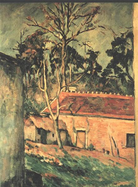
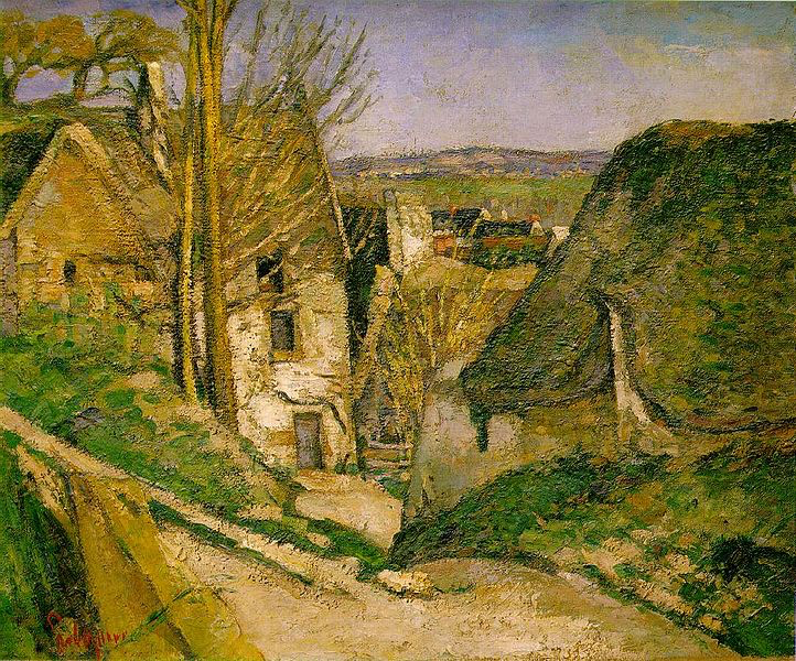
These two pictures are both by Paul Cezzane. In Cutting’s research, the picture on the right was found to be reproduced in literature 165 times while the picture on the left was reproduced only 30 times. When shown side by side, the test subjects preferred the picture on the right by a 65% margin.

Overall, consistent with other tests examining the Mere Exposure Effect, Cutting found that 59% of the variation in aesthetic judgement could be explained by looking at the logarithm of the frequency of base exposure to the picture (Cutting, 2003).

However, just using this test alone presents a problem. Certainly, the subjects judged the most published artwork as the most beautiful. But, that finding alone does not sufficiently prove exposure is what caused these judgements. Perhaps the reason these artworks were the most published to begin with was because they were somehow the most beautiful (cum hoc ergo propter hoc)?

To test for just this possibility, Cutting proceeded to do another test with a different cohort of subjects. In this test, Cutting somewhat randomly exposed a classroom of 116 subjects to the same set of images. However, over the course of a semester, Cutting exposed his subjects to the least published images four times more than the most published images. At the end of the semester, Cutting found his subjects now preferred the more published images relatively less often, with a correlation of only 48% to the logarithm of base exposure.

For 41 of the 51 pairs, in fact, the preference for the most published image went down. In the case of the Cezanne pictures above, the aesthetic preference for the most published image (the one on the right) went from 65% to 63%. In one case, the preference for the most published image went from down by 41% after the lesser published image was shown more often to the subjects.

In other words, by exposing his subjects more often to the less published images, Cutting was able to reverse the preferences in a statistically significant way.

Both of these test findings support the hypotheses that the “fittingness” of a painting can be tested by looking to understand the frequency of that painting in the memory of subjects and that the paintings more frequent in their memory would be judged to be more beautiful.

Computational Psychology Grounding for Effort

Given that we are looking at agent memory for our model, we decided to look to the Adaptive Control of Thought – Rational (ACT-R) algorithm used in cognitive computational psychology (Anderson & Milson, 1989). Specifically, we adopted a variant of a model optimized by Alexander Petrov for computational simulations (Petrov, 2006, Equation 2).

The ACT-R algorithm takes the logarithm of the frequency of exposures and modulates this using several other variables to derive an “arousal” value. We use this arousal value to have agents choose between two paintings.

Equation 1. Petrov revised ACT-R algorithm for computational simulation

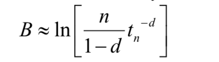
In this equation, n is the frequency of exposure, t is the time since the i-th activation and d is the decay rate of activation. For the purposes of this project, we note that the generally accepted value in the literature for d is 0.5 (Petrov, 2006), but we will test 0.4 and 0.6 as well.

Pseudo Code for Model

1. “Replicate” Cutting’s experiment (null hypothesis):
   1. Create a virtual classroom of agents (i.e., subjects)
   2. Create an inventory of paintings with a base exposure frequency for each painting (in this case, the exact names and base publication frequencies for the actual Cutting test are used to establish the base inventory)
   3. At Tick 1, find the correlation (the R value) between paintings’ base exposure frequency and the ACT-R activation value for each painting
   4. Fill each agent’s memory with the inventory of paintings and their base exposure frequencies
   5. Randomly show the agents paintings from the inventory (at an initial ratio of 1:4 times for the most published/least published painting). Allow this ratio variable to be changed through a slider (Ratio of More:Less)
   6. Have each agent update their memory and ACT-R value as paintings are viewed additional times
   7. Tick / Repeat from Step E until run is set to end.
   8. Test for the correlation (the R value) between the base exposure frequency and choice over all painting pairs. As agents are more exposed to the less published images, this correlation should go down.
   9. Make the agents heterogeneous. Give agents different frequency distributions and ACT-R values for paintings.
   10. Allow for more granular representations of paintings (e.g., characteristics and traits) (Axelrod, 1997)
2. Introduce a “tastemaker” that impacts the frequency of paintings in agent’s memories
   1. Choose an agent to be tastemaker. At setup ask the tastemaker to choose a random painting as the tastemaker’s favorite.
   2. At each tick, have the tastemaker “promote” their favorite painting to the other agents and then have that painting replicated X times in agent memory (as set by a slider, “Tastemaker Impact”)
   3. Test for the correlation (the R value) between the base exposure frequency and choice over all painting pairs
   4. Test what happens when the tastemaker only promotes various paintings among the most published works in the inventory (top quartile)
   5. Test what happens when the tastemaker only promotes various paintings among the least published works in the inventory (bottom quartile)
   6. Test what happens when the tastemaker only sporadically promotes specific artwork (this should be about the same as reducing the Tastemaker Impact slider)
3. Spatialize the model
   1. Make agents heterogeneous
   2. At intervals, decide what is the favorite painting of a neighborhood and then add an extra N copies of that painting to the neighborhood’s memories

Discussion of Findings

In its present state, the model does not predict the actual values observed in Cutting’s subject for his test where he showed his subjects less published paintings four times more than published paintings. However, there is a rough congruence in the distribution of selections.

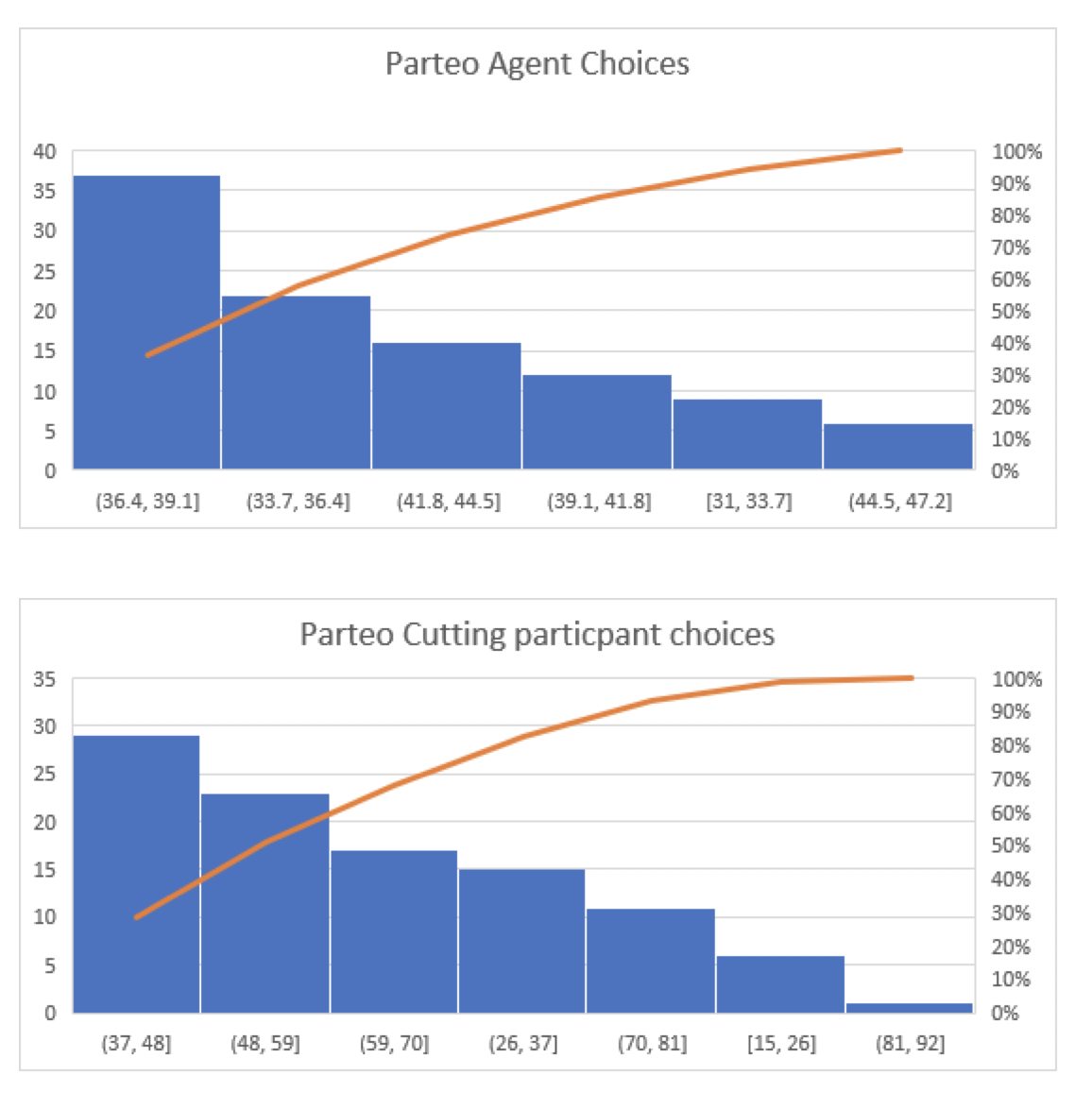
Figure 3. Comparison of preference distributions between Cutting’s findings and model’s findings

We hypothesize that, over many runs, when agents are more exposed to paintings that had a lower base level of publication, the correlation between agents’ preferences for the paintings that were less published initially would increase. This was not, in fact, what we found.

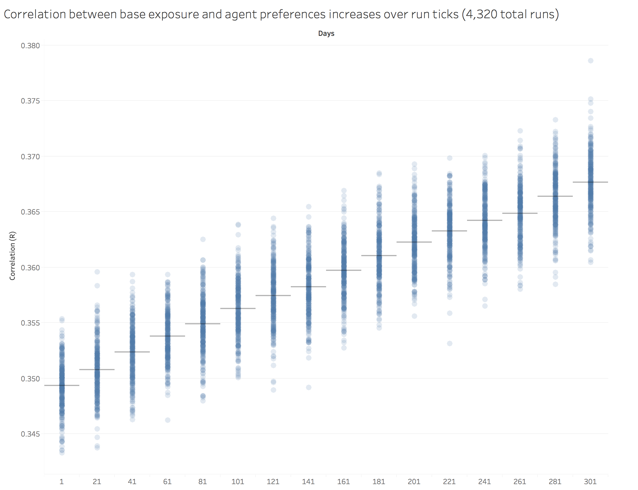
Figure 4. The longer the model run, the higher the correlation of preferences with the most published paintings. Each dot is the result of a single run, bars indicate the mean of the runs for the independent variable.

Next, we tested for what would happen if we varied the relative ratios of exposure between lesser published and more published paintings. We hypothesized that the greater the ratio of exposure to less published paintings, the less often agents would choose the more published paintings. To our chagrin, this was not the model’s result.

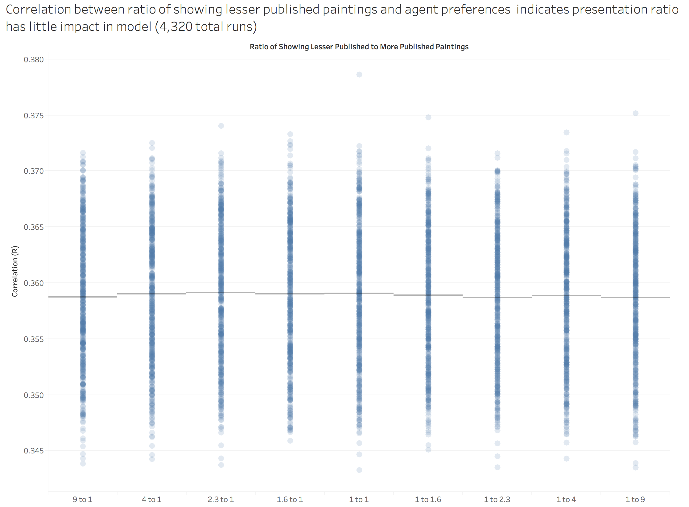
Figure 5. Model results not significantly impacted by varying ratios of exposures. Each dot is the result of a single run, bars indicate the mean of the runs for the independent variable.

Next, we chose to investigate the impact of changing the decay rate of the ACT-R algorithm used by our agents. We were not sure what the effect would be. We found that varying the decay rate had little impact on the correlation of preferences.

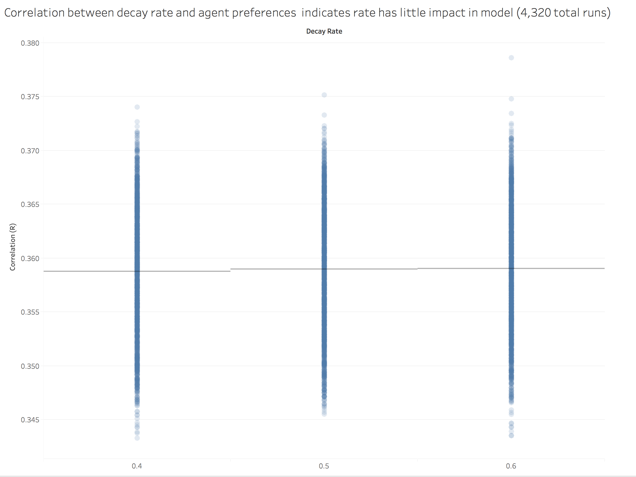
Figure 6. Model results not significantly impacted by changing ACT-R decay rate value. Each dot is the result of a single run, bars indicate the mean of the runs for the independent variable.

Finally, we introduced the idea of a Tastemaker. The Tastemaker is an agent that randomly selects and promotes a specific painting to all other agents who then update their memory to add an additional X copies of the painting (as set by a slider). Our overall findings indicate that, for future versions of the model, we would want to have the tastemaker promote more than one specific painting and test for what would happen if the tastemaker choses less published or more published paintings to promote.

We would hypothesize, all else being equal, that over time the influence of the tastemaker would decrease the correlation between agent preferences. As shown below, that is not what we found.

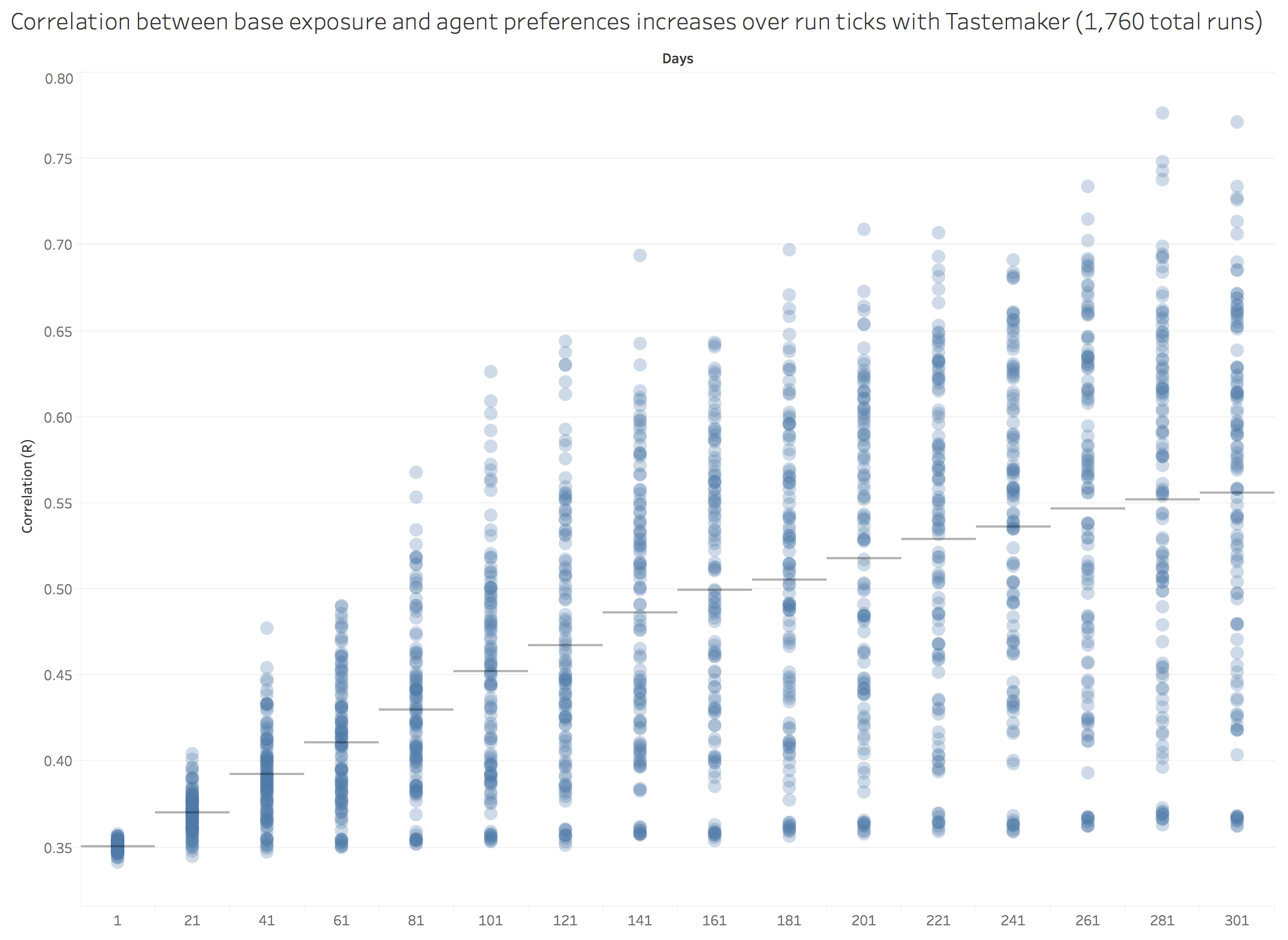
Figure 7. Adding a Tastemaker results in overall higher correlations contrary to initial hypotheses. Each dot is the result of a single run, bars indicate the mean of the runs for the independent variable.

To further test the model, we examined what would happen if we varied the number of times a promoted painting was put into the memory of all the agents. This variable is termed “Tastemaker Impact.” We caution that we have work to do on this part of the model in that the tastemaker only promotes a single, randomly drawn, painting. Nonetheless, we did discover a strong impact between this variable and the correlation of agent preferences as shown below.

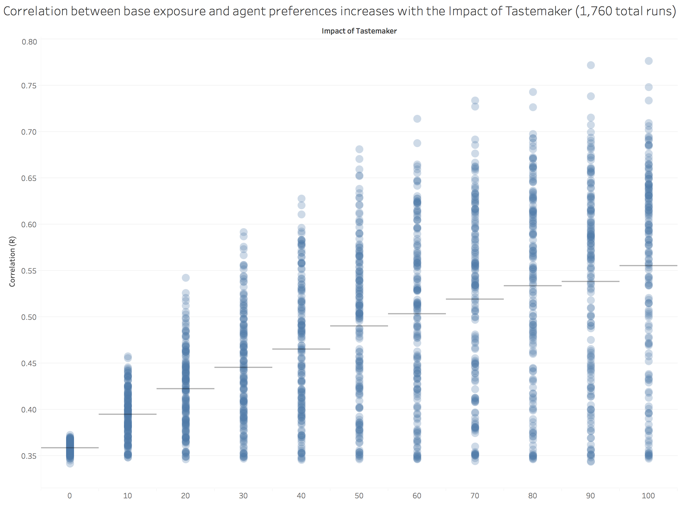
Figure 8. Increasing Tastemaker Impact results in overall higher correlations. Each dot is the result of a single run, bars indicate the mean of the runs for the independent variable.

Finally, we examined how both varying Tastemaker Impact and time impacted the correlation of agent preferences. For the most part, the relationship of these variables remains fairly constant with our previous findings.

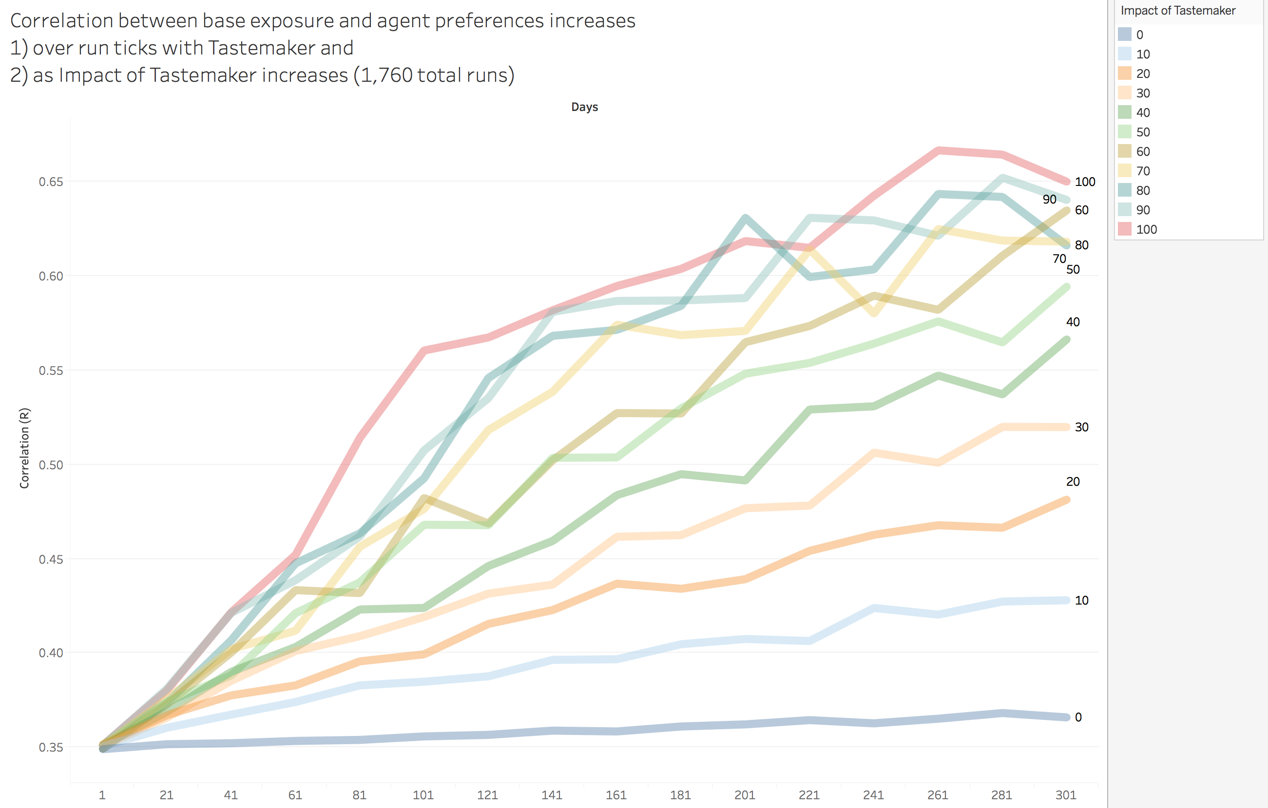
Figure 8. For the most part, the correlation of agent preferences and Tastemaker Impact holds fairly constant over the time of the run. Each line represents the correlation over time for different values of Tastemaker Impact.

If you, like us, believe that the ultimate measure of an analytical effort is not the answers gained, but instead the discovery of new questions to be asked, we believe that this effort has been a resounding success. We are ready to declare victory on that front. The results that we obtained from the present version of the model diverge so much from what we would expect, we believe that even more verification of the model needs to be done and points the way for future improvements.

Limitations of Findings

Our approach has a number of constraints and limitations but has helped us to ask better questions.

1. To the extent that beauty can be found independently of something being more liked, testing for the influence of the Mere Exposure Effect has intrinsic boundaries.
2. At some point, experimental psychology has found that liking can actually decrease after some point in time with repeated exposures (Montoya, Horton, Vevea, Citkowicz, & Lauber, 2017). For simplicity, we choose not to address that in our model. I personally find it humorous that one study found, that with bad art, repeated exposures never increased liking and actually increased disliking (Meskin, Phelan, Moore, & Kieran, 2013). While these dynamics are very amenable to computational modeling, for simplicity sake, we chose not to fully try to model this dynamic.
3. If fittingness indeed drives aesthetic judgement, it should be recognized that fittingness is multi-dimensional and driven by much more than the instant feeling one gets from looking at an image (Nanay, 2017). As noted before, the human mind likes to find patterns and the patterns found by looking at art extend far beyond the image itself. Every artwork is framed by an observer-dependent context that is informed by that observer’s memory and cognitive processes.
4. For all of our efforts to posit that there is deterministic mechanism that can influence aesthetic judgements, we are willing to admit, and indeed hopeful, that beauty itself might go beyond deterministic factors.
5. Our approach considers artwork traits as “categorical.” What this means is that, for our approach, a trait with a value of 11 is as different from a trait with a value of 99 as it is with a trait of a value of 12. What if instead, things are actually more graduated, and instead of categorical values, our trait values represented “intervals?” For example, what if a trait represented a color? Agents who liked value 11 would likely be more prone to like value 12 than value 99. After a fairly lengthy examination of this dynamic, which included reaching out to math professors on campus, we were unable to come up with a satisfactory algorithm to address that dynamic. For more on this limitation, see Appendix A.

As an observation, not as a criticism, we note, for example, that in Axelrod’s iconic cultural model (Axelrod, 1997), similarity between cultures is calculated by categorical similarity. The similarity of cultures is determined by how many trait values are exactly identical. Perhaps Axelrod would have gotten different results if he measured the similarity of cultures by treating trait values as interval values instead?

1. As a continuation of the last issue, it is questionable that a painting can be reduced to a set of interval values. The authors of this paper are divided on this question. To Paul, the reflexivity inherent in art judgement between pieces of art and the multi-dimensional nature of the judgements make this effort doomed to failure. However, Paul believes that we might be able to come close enough to ask valuable questions by coming up with random values to use in representing characteristics and traits of a painting. Fahad thinks that we can actually begin with an empirical set of paintings and quantify them sufficiently for a study. Fahad reminds us that a jpeg, for example, is an example of just such a process as reducing an image quantitatively.

Conclusion

Beauty might indeed lie in the eye of the beholder. We argue that a painting’s perceived beauty is very often a function of the fittingness of that painting with the beholders memory. Using the analytical tools offered by ABM and based on grounding in Experimental and Computational psychology, this paper lays the groundwork for such an exploration.

We suggest that a fittingness function be looked at much more often in the field of ABM and hope that our efforts have helped, at least dimly, light such a direction.

Bibliography

Anderson, J. R., & Milson, R. (1989). Human memory: An adaptive perspective. Psychological Review, 96(4), 703–719. https://doi.org/10.1037/0033-295X.96.4.703

Axelrod, R. (1997). The Dissemination of Culture: A Model with Local Convergence and Global Polarization. Journal of Conflict Resolution, 41(2), 203–226. https://doi.org/10.1177/0022002797041002001

Barabasi, A.-L., & Bonabeau, E. (2003). Scale-Free Networks. Scientific American, 288(5), 60–69.

Beinhocker, E. D. (2006). The origin of wealth: evolution, complexity, and the radical remaking of economics. Boston, Mass: Harvard Business School Press.

Bornstein, R. F. (1989). Exposure and affect: Overview and meta-analysis of research, 1968–1987. Psychological Bulletin, 106(2), 265–289. https://doi.org/10.1037/0033-2909.106.2.265

Cunningham, M. R. (1986). Measuring the physical in physical attractiveness: Quasi-experiments on the sociobiology of female facial beauty. Journal of Personality and Social Psychology, 50(5), 925.

Cutting, J. E. (2003). Gustave Caillebotte, French Impressionism, and mere exposure. Psychonomic Bulletin & Review, 10(2), 319–343. https://doi.org/10.3758/BF03196493

Cutting, J. E. (2007). Mere exposure, reproduction, and the impressionist canon. Partisan Canons (Durham, NC: Duke University Press) Pp, 79–93.

Cutting, J. E. (2017). Mere Exposure and Aesthetic Realism: A Response to Bence Nanay. Leonardo, 50(1), 64–66. https://doi.org/10.1162/LEON_a_01081

Epstein, J. M., & Axtell, R. L. (1996). Growing Artificial Societies: Social Science From the Bottom Up (First edition). Washington, D.C: Brookings Institution Press & MIT Press.

Falk, J. H., & Balling, J. D. (2010). Evolutionary Influence on Human Landscape Preference. Environment and Behavior, 42(4), 479–493. https://doi.org/10.1177/0013916509341244

Hodder, I. (2012). Entangled: an archaeology of the relationships between humans and things. Malden, MA: Wiley-Blackwell.

Hodder, I. (2016). Studies in Human-Thing Entanglement. Retrieved from http://www.ian-hodder.com/books/studies-human-thing-entanglement

Langlois, J. H., & Roggman, L. A. (1990). Attractive Faces Are Only Average. Psychological Science, 1(2), 115–121.

Meskin, A., Phelan, M., Moore, M., & Kieran, M. (2013). Mere Exposure to Bad Art. The British Journal of Aesthetics, 53(2), 139–164. https://doi.org/10.1093/aesthj/ays060

Montoya, R. M., Horton, R. S., Vevea, J. L., Citkowicz, M., & Lauber, E. A. (2017). A re-examination of the mere exposure effect: The influence of repeated exposure on recognition, familiarity, and liking. Psychological Bulletin, 143(5), 459–498. https://doi.org/10.1037/bul0000085

Nanay, B. (2017). Perceptual Learning, the Mere Exposure Effect and Aesthetic Antirealism. Leonardo, 50(1), 58–63. https://doi.org/10.1162/LEON_a_01082

Petrov, A. A. (2006). Computationally efficient approximation of the base-level learning equation in ACT-R. In Proceedings of the seventh international conference on cognitive modeling (pp. 391–392). Citeseer.

Reber, R., Schwarz, N., & Winkielman, P. (2004). Processing Fluency and Aesthetic Pleasure: Is Beauty in the Perceiver’s Processing Experience? Personality and Social Psychology Review, 8(4), 364–382. https://doi.org/10.1207/s15327957pspr0804_3

Rigau, J., Feixas, M., & Sbert, M. (2008). Informational Aesthetics Measures. IEEE Computer Graphics and Applications, 28(2), 24–34. https://doi.org/10.1109/MCG.2008.34

Zajonc, R. B. (1968). Attitudinal effects of mere exposure. Journal of Personality and Social Psychology, 9(2, Pt.2), 1–27. https://doi.org/10.1037/h0025848

Appendix A: Challenges in representing artwork for modeling purposes

Suppose we have a given artwork “Y” that is represented as “01 11” and a given agent’s memory as “08 11” and “02 11.” Each artwork has two characteristics (number positions) and each characteristic is given has a trait value.

We could hypothesize that an artwork’s quantification reflects a categorical value; that 08 11 and 02 11 are both equally different from 01 11 because they both have one characteristic that is different from the referent 01 11. This would be equivalent to taking the Hamming Distance from the referent to each artwork in memory.

In theory, this approach would most closely replicate Cutting’s tests.

However, it might not be that simple. Each characteristic’s trait value might not be a unique value but rather a value that lies on a continuum. Suppose the first position represents dominant color and 01 represents the color Blue.

Repeatedly exposing agents not to the exact color Blue (01), but similar values (say 00 and 02), could increase the agent’s appreciation of “blueness.” To consider this effect, we would want to treat each trait value as an interval value versus treating each trait value as a unique categorical value.

If we wanted to treat a painting’s trait value as a categorical value, one would be tempted to look in each agent’s memory and find the modes of each characteristic.

For example, suppose Agent 5 had the following values for Characteristic 1 with the following frequencies in their memory (size 100):

Characteristic 1 Value	Frequency
11	40
02	32
01	28

Now, let’s suppose we have a new referent artwork to evaluate whose Characteristic 1 is 03.

The question to ask is do we evaluate “03” as a difference in category value, in which case “03” is equally different from all the values in memory, or a difference in interval value, in which case “03” is less different from the values “02” and “01” than from the value “11?”

Suppose, for now, we want to test our referent number for differences in interval value.

The mean of Agent 5’s memory, as shown above, is 5.28. If we wanted to consider how distant “03” is from all the values in Agent 5’s memory, it is tempting to ask how “03” compares to that value.

However, if instead, we created a row in a spreadsheet for each memory value, and then tested X values as a new referent X(0,20) and asked how distant X was from each memory in memory (absolute(reference number – memory number) and then summed these values to find Total Distance, we would find that it is not when the referent number approaches the mean of the values that Total Distance is minimized.

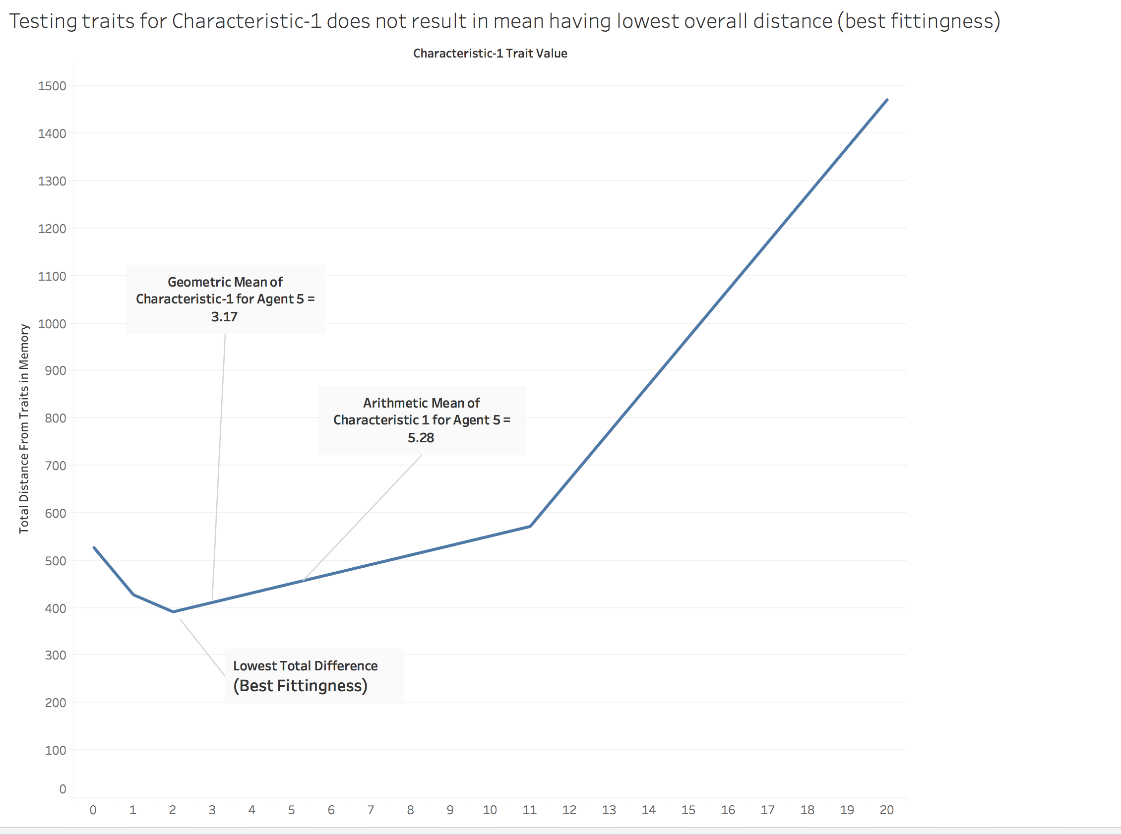
Figure 9. Sample value with the lowest total distance from sample distribution not arithmetic mean and not the geometric mean.